
Jon David Groff (@JonDavidGroff), part of the #GameMyClass crew, asked about random dice roll sites the other day on Twitter. It got me thinking of the random number generator on Excel and Google Sheets. A dice roll is really nothing more than a randomly generated number with a set boundary. a D20 roll will return a random number between 1 and 20 for example. This then led me to think about incorporating a Random Number Generator (=RANDBETWEEN) with the vlookup (=VLOOKUP) function to return an image paired to the randomly generated number. Since I consider myself an Enthusiastic Amateur Spreadsheeter I thought I’d take a shot at making a Dice Roll Spreadsheet.
Feel free to make a copy, make improvements, and share it back: Dice Roll Spreadsheet (Force Copy Edition)
“How To” Outline
- First Create a Google Sheet. I started with 2 tabs. The first was for the Dice Roll (originally called 1 Die) the second was for the D20 images.
2. Make the Images for the dice roll possibilities using Google Draw.

3. Publish the Graphic to the Web by clicking the File -> Publish to the Web


4. Add the Publish to the Web Link in the appropriate location on a Table in the D20 Tab. Your tab might be for a D6 or D10 but the principle is the same. Create a 3 column table. Column A is the possible dice roll outcome. Column B is the published web link. Column C is the function =image(B_) where the cell is the publish web link you would like displayed.


5. Repeat this process of adding the Published Web links until all of image possibilities are on the table. to save some time write the =image function once and then click and hold the little blue box on the bottom right of the cell. While holding down on the little blue box drag the function down to the last possible outcome. It will automatically change the cell in the function.
Now turn to the sheet where you would like the Dice Roll to take place. I named mine 1 Die.
Create the Random Number Generator
I made my function a little complicated. The simplest way is to just add the function =RANDBETWEEN(1,20). The numbers in the function represent the lower and upper range. If you want a D6 roll the function would be =RANDBETWEEN(1,6). With this simple function any time a cell anywhere on the sheet is changed a new number within that range will be generated.
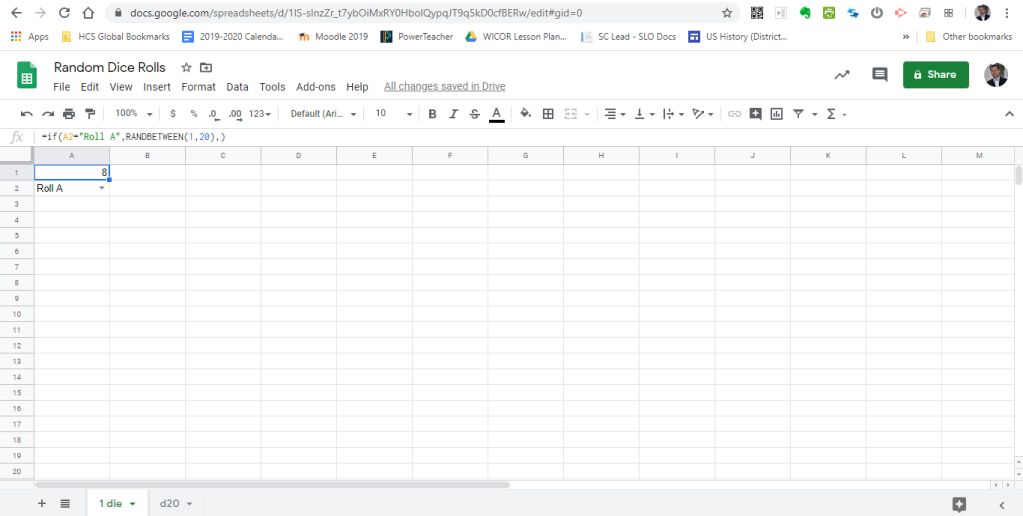
I wanted to create a single cell that would create to the random number generation. So I added a Data Validation Cell A2. This creates a drop down menu with a limited number of choices. To test this concept I made two options – “Roll A” and “Roll B”. To create a Data validation click on the cell to validate and then click on file -> data validation.

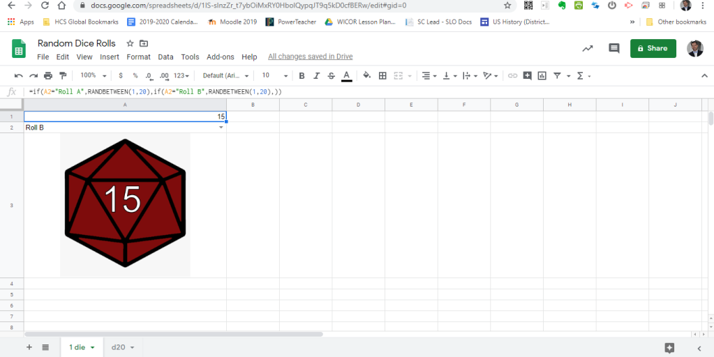
With the dropdown menu in place mashup the “RANDBETWEEN” with a “NESTED IF” function. This will allow the random number to be generated when either of the 2 functions is clicked and it will return a blank cell if neither is clicked. The function is =if(A2=”Roll A”,RANDBETWEEN(1,20),if(A2=”Roll B”,RANDBETWEEN(1,20),)). (For more on “Nested Ifs” check out his previous post = https://classroompowerups.com/2018/06/11/more-g-sheets-magic/)
Return the Dice Image with VLOOKUP
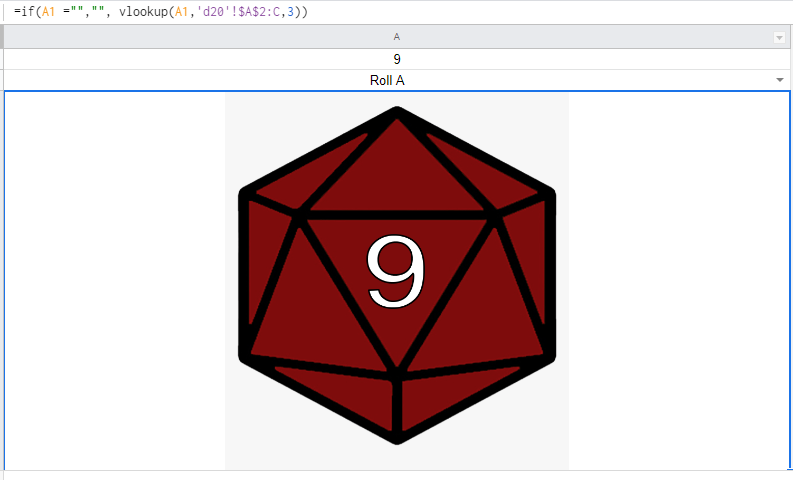
In the cell where the image is to be displayed use the function =if(A1 =””,””, vlookup(A1,’d20′!$A$2:C,3)). The function is saying that IF there is ANY VALUE ( represented by “,”) in cell A1 then use the vlookup formula in the function. the vlookup function says to use the number in A1 and find that value in the table located in tab d20. the Table starts at cell A2 (shown here as $A$2) and will continue over to column C. The function looks for the value on the farthest left column (here it is A); so the value in cell A1 from the ‘1 die’ tab will be found in column A of the ‘d20’ tab. When the value is found the function needs to know what value to return. The “3” tells the function to return the value in the 3rd column in the chart; in this case column C. Since column C is our image function the function will place the image into the cell in the ‘1 die’ tab where we have wrote the original function. Complicated right? This is what it looks like.
Play around with your own copy to see how it works. I am certain improvements can be made! I would love to see them.
UPDATE: Since this original writing I have added a 2 d20 dice roll

Hi!! I absolutely love your tool! I adopted it and added extra hyperlinks to make the rolls happen on demand from within my character sheet. I also adjusted the rolls to be D10s, but that was EzPz once i noticed that you used Randbetween. One question though: How did you make the Dice Roller pages have only the REQUIRED amount of columns and rows? For example, for the 1d20, you have only Column A, and Rows 1,2,3. I wanted to do the same with my Custom Character sheet for WoD that i’ve built on Google Sheets, but can’t seem to find how. Any suggestions?
LikeLiked by 1 person
If I understand what you’re asking it’s pretty simple – just delete all of the other column and rows. Click the row you want to star at and drag all the way to row 1000 and then delete. Do the same with the columns.
LikeLiked by 1 person